Date - 11/08/2026
Our plan for this session was to complete the remaining half of Andrej Karpathy’s makemore part 1, which reframes the counting bigram model from Session Two as a neural network.
We changed direction again before we started. That second half opens by calling loss.backward() and stepping the weights, and neither of those means anything without a working grasp of how gradients are computed. Reading the code would have been possible; understanding it would not.
So we spent this session on Andrej Karpathy’s The Spelled-Out Intro to Neural Networks and Backpropagation: Building micrograd instead. It builds a tiny automatic differentiation engine from nothing, then builds a small neural network on top of it. It is the missing prerequisite rather than a diversion.
Why we changed direction
Session Two deliberately stopped at the counting model: probability tables, sampling, negative log likelihood, and no learning of any kind. Training there meant walking the dataset once and tallying.
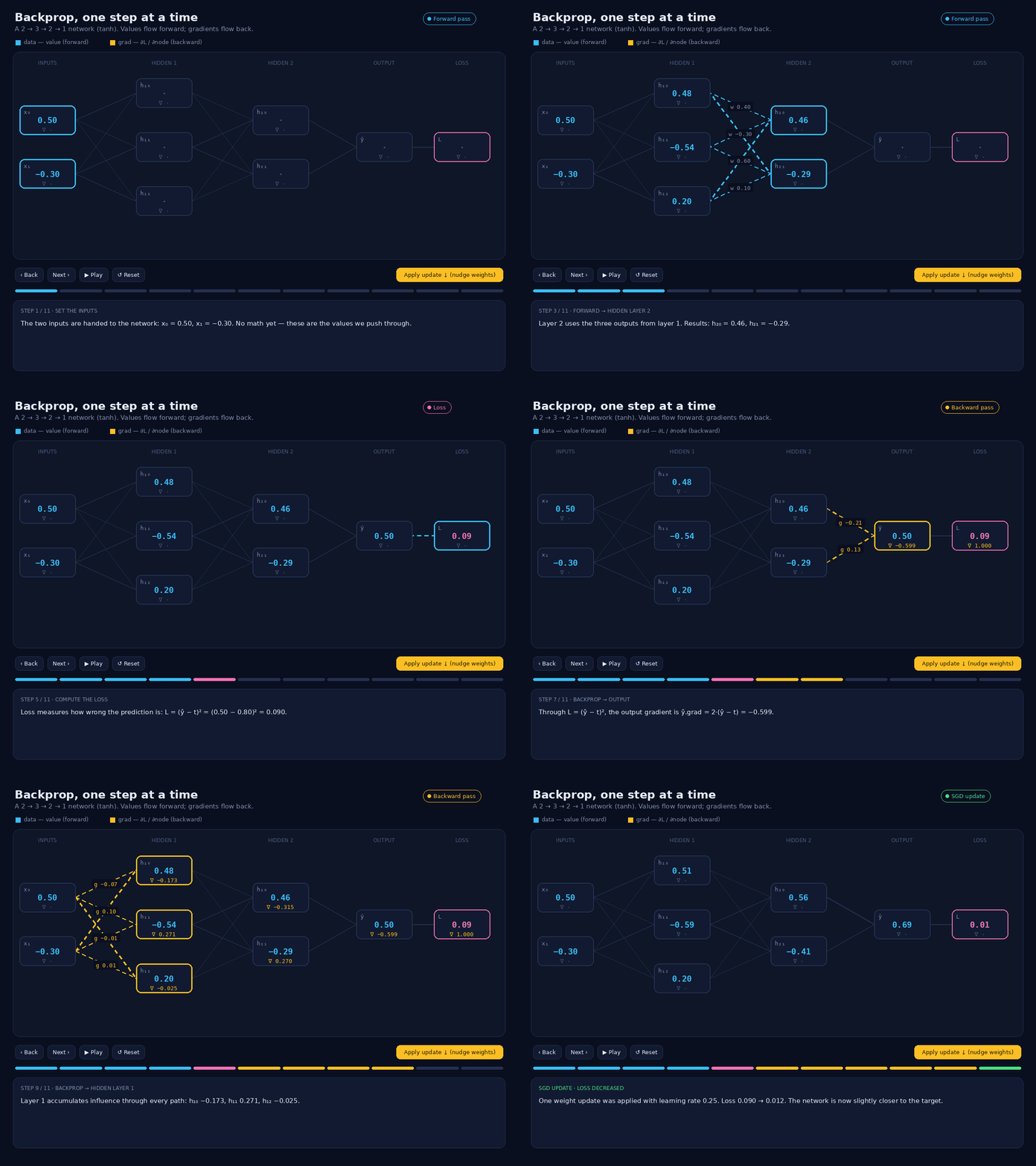
Everything after that point in the series involves the same four steps repeated many times over: forward pass, loss, backward pass, update. Backpropagation is the third of those, and it silently underpins every model we will look at from here to the Transformer.
The judgement we made was that one session spent on backpropagation would make the following four sessions comprehensible rather than memorised, so it was worth the delay. It remains a timeboxed detour. The destination is still the application layer.
What we covered
The video has two halves, and so did the session. The first half builds a computation graph and performs backpropagation across it. The second half assembles a small neural network out of that same machinery. The hardest conceptual jump is the hierarchy that emerges by the end: values, then neurons, then layers, then a multi-layer perceptron.
The Value object
Every single number in the graph is a Value object rather than a plain float. Each one stores four things:
data— the number itself, produced during the forward passgrad— the derivative of the final output with respect to this value, filled in during the backward pass and starting at zero- the operation that created it (
+,*,tanh, and so on) - pointers to its parent nodes, which are the values that produced it
The parent pointers are what make backpropagation possible at all. Without them there is no trail to follow backwards from the output to the inputs.
Building the graph
Writing d = a * b + c does not simply produce a number. Each operation creates a new Value node that records which operation made it and which values were its parents. The node produced by a * b knows that it came from a multiplication and that its parents were a and b.
That stored operation is exactly what tells the backward pass which local derivative rule to apply later.
Local derivatives and the chain rule
The central insight of the first half is that each node only needs to know its own local derivative. No node ever needs a view of the whole graph.
Addition passes the incoming gradient straight through, unchanged. Multiplication swaps in the other input. The tanh node multiplies by 1 - tanh(x)**2.
The chain rule then stitches those local pieces together into the full derivative. At every node the calculation is the same: the local rule multiplied by whatever gradient arrived from behind.
Forward pass and backward pass
Obtaining a gradient is a two-pass process.
The forward pass feeds inputs in and computes left to right until the final output. The graph records every operation and every value along the way. At the end of it we have all the data and no gradients.
The backward pass starts at the very end, seeds the final node with a gradient of one, then walks backwards applying each node’s local rule multiplied by the incoming gradient. This fills in grad on every node in the graph.
The seed value of one is worth stating precisely, because it is easy to misread. The output’s derivative with respect to itself is one. It has nothing to do with the numerical value of the loss.
The manual nudge demonstration
Before the neural network appears, there is a small demonstration of the idea of learning. Run the backward pass to obtain each input’s gradient, then move every input a little in the direction of its gradient. The output goes up, exactly as the gradients predicted.
The update rule for each input is:
new data = old data + (step size × grad)
Multiplying by the gradient rather than only using its sign matters for two reasons. Size is information: a large gradient means a strong effect, so that input should move further. And the sign takes care of itself, because a negative gradient makes the whole term negative and the input moves down without anyone reasoning about direction.
This is learning in miniature. The gradient supplies the direction, and a small step moves along it. In real training the step is taken in the opposite direction so that the loss goes down, which is what gradient descent means.
The artificial neuron
A single neuron multiplies each input by its weight, sums the results, adds a bias, and squashes the total through an activation function:
y = tanh(w1*x1 + w2*x2 + ... + b)
A neuron holds one weight per input plus exactly one bias, which means a neuron with three inputs owns four values, and one with two inputs owns three. It is not a single number.
Internally the neuron builds the same multiply-then-add graph from the first half of the session, feeding into a final tanh node. The building blocks do not change; only the arrangement does.
The distinction between the two levels is worth keeping clear. A Value is a low-level graph node, one per weight and one per intermediate result. A Neuron is a container that owns a bundle of those values. The neuron does not replace the value; it holds a handful of them.
Activation functions
tanh squashes its input into the range −1 to 1, and sigmoid squashes into 0 to 1. Squashing the range is the visible behaviour, but it is not the real reason activations exist.
Without an activation, stacking layers achieves nothing. A chain of linear steps collapses into a single linear step, so the network can only ever draw straight lines. The activation introduces a bend at each layer, and that bend is what allows the network to represent curves and more complicated shapes.
For following the code, “it squashes into a range” is an adequate working description. The non-linearity is the footnote that matters later.
Neuron, Layer, and MLP
The second half is three classes, each containing the previous one, and each with the same three methods.
A Neuron creates its weights and bias as random values in its constructor, computes w·x + b followed by tanh when called, and returns its weights and bias from parameters().
A Layer is a row of neurons side by side. Its constructor takes the number of inputs and the number of neurons and builds them. When called, it feeds the same inputs to every neuron and collects one output from each, so five neurons produce five outputs. Its parameters() gathers the weights and biases of all its neurons.
An MLP, or multi-layer perceptron, is a stack of layers in sequence. Its constructor takes the layer sizes and builds them. When called, it passes the inputs through each layer in turn, with one layer’s outputs becoming the next layer’s inputs, and the final layer’s output as the answer. Its parameters() gathers every weight and bias in the whole network.
The hierarchy in one line: an MLP is a list of layers, a layer is a list of neurons, and a neuron is a bundle of values.
__call__ and why the code reads so cleanly
__call__ is a standard Python dunder method rather than anything specific to micrograd. Defining it makes an instance callable in the same way as a function:
n = Neuron(2)
out = n(x)        # runs n.__call__(x)
Because of this, a layer can invoke each of its neurons with neuron(x), and an MLP can invoke each of its layers the same way. Everything in the hierarchy becomes callable, so the code reads as data flowing through a chain of functions rather than as objects being manipulated.
Why parameters() exists
Training requires reaching every weight and bias in order to nudge each one. parameters() is the convenient list of everything that is allowed to be tuned, gathered up the hierarchy from neuron to layer to network. It is the same list that the training loop will iterate over in the next session.
Next session
We return to makemore and finish the second half of part 1, rebuilding the bigram model as a one-layer neural network.
That means one-hot encoding, a weight matrix, logits, softmax, negative log likelihood as a loss, and gradient descent doing the work that counting did in Session Two. The expectation is that it arrives at roughly the same result as the counting model, and the interesting question is why the more complicated route is worth taking.
Resources
- Andrej Karpathy — The Spelled-Out Intro to Neural Networks and Backpropagation: Building micrograd
- micrograd repository